Some vehicles cannot operate on their own but rather depend on additional shared assets to execute their routes. These assets are called resources. A resource can represent anything such as a driver, trailer or a specialized piece of equipment.
The optimization will assign resources to routes in such a way that total cost is minimized. This includes both the individual cost of each route and any additional cost associated with using specific resources. When multiple vehicles are assigned the same resource, the algorithm ensures their routes are separated in time, potentially with a buffer in between. This allows limited resources to be shared efficiently, without violating timing or exclusivity constraints.
Buffer duration
When multiple vehicles share the same resource, back-to-back scheduling can cause conflicts or delays if the resource isn’t ready immediately after use. Defining a minimum buffer duration on a resource solves this by enforcing a minimum time gap between assignments. For example, a trailer needing cleanup after each route can have a buffer time to ensure it’s prepared before its next usage.
Costs
Resource costs are structured to capture different aspects of using shared assets. These costs fall into four main categories:
- Fixed costs - Represent one-time expenses incurred when a resource is used.
- Per-vehicle costs - Reflect charges applied each time a resource is assigned to a vehicle route.
- Over-vehicles costs - Threshold based costs add extra fees when the number of vehicles using a resource exceeds certain limits.
- Layover costs - Represent a cost incurred for every layover that is scheduled.
Together, these cost types provide flexibility to model a wide range of operational and financial considerations for resource allocation.
Fixed cost
A fixed cost is a one-time expense incurred whenever a resource is used, regardless of how many vehicles it supports. Its primary purpose is to encourage minimizing the total number of different resources utilized. By assigning a fixed cost, the optimization naturally favors reusing the same resources across multiple routes rather than starting new ones, helping to reduce overall resource count. For example, in an AM/PM driver scheduling plan, fixed costs can be applied to driver resources to minimize the total number of drivers needed throughout the day, promoting efficient shift assignments.
Per-vehicle cost
Per-vehicle costs are charges applied each time a resource is assigned to a vehicle route. Their main purpose is to limit how often a particular resource is used by increasing the cost with each additional assignment. This helps control workload or restrict overuse of resources that might be costly or limited in availability. For example, if vehicles represent daily tasks and resources represent trucks, some trucks may be rented rather than owned. Applying per-vehicle costs to these rented trucks encourages the system to minimize their use and prioritize owned trucks whenever possible.
Over-vehicle costs
Over-vehicle costs allow for more advanced and flexible cost modeling by introducing thresholds that trigger additional charges when a resource is assigned to more vehicles than a defined limit. This enables planners to represent more nuanced or escalating cost structures, such as capacity strain, wear-and-tear, or operational inefficiencies that grow with overuse. A typical use case is fleet balancing—where all resources (e.g. drivers or trucks) should be utilized evenly across the plan. By setting multiple thresholds with increasing costs, the system is discouraged from assigning a single resource to many vehicles while others remain underused. For instance, if one resource is used four times while another is only used once, these escalating costs can push the optimizer toward a more balanced and equitable distribution.
Layover costs
Layover costs are applied when a resource stays at a designated layover location between consecutive routes instead of returning to its home base. These costs can represent driver accommodation, allowances, or vehicle parking expenses. Including a layover cost allows planners to reflect the trade-off between returning home and remaining in the field, helping the optimization model decide when scheduling a layover is appropriate based on overall cost efficiency.
Constraints
To manipulate the group of vehicles that share a resource, constraints can be defined to limit resource usage. The following constraint types are currently supported:
- Maximum vehicles - Specifies the maximum number of vehicles that can be assigned to a single resource. Example: When modeling drivers as resources, this constraint can enforce that a driver is assigned to no more than a specified number of vehicles.
- Maximum total route duration - Specifies the maximum cumulative duration of all routes assigned to vehicles sharing the same resource. Example: Useful for modeling driver work limits, where a driver (resource) can only work for a certain number of hours in total.
Example: limit driver shifts
Say driver "John" may work at most 40 hours a week and 5 days out of 7. John also needs to take a daily rest of at least 11 hours. To model this use case, we can create 7 vehicles (one for each day of the week) and require "John" as a resource on each of these. The resource "John" can then be modelled as:
"resources": [
  {
    "id": "John",
    "minimumBufferDuration": 39600,
    "constraints": {
      "maximumVehicles": 5,
      "maximumTotalRouteDuration": 144000
    },
    "categories": [
      "driver", "John"
    ]
  }
]
Categories
Categories allow resources to be grouped by type or physical characteristics, such as "driver", "truck", or "pallet-jack". Instead of assigning specific resources to vehicles, the system lets vehicles require a resource from a given category.
For example, consider a scenario where resources represent trailers. All vehicles require a trailer to operate, but some vehicles specifically need trailers with cooling capabilities. In this setup, all trailer resources share the category "trailer", while only those equipped with cooling also have the additional category "cooling". Vehicles that require refrigeration can request a resource from the "cooling" category, while others simply request a "trailer". This setup allows a cooling trailer to be used flexibly—either in cooled mode when required or as a regular trailer when cooling isn't needed.
Examples
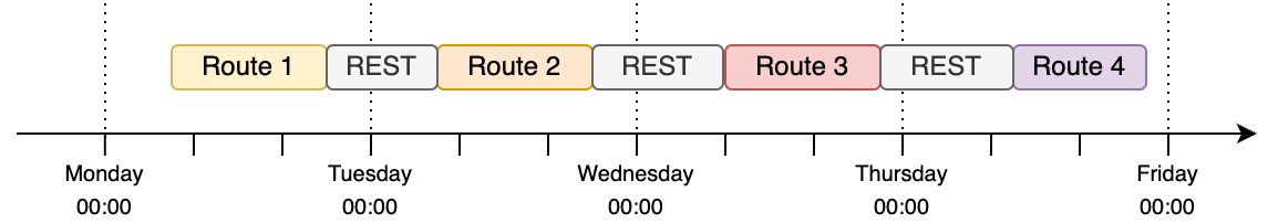
Daily rest rules
In this scenario, we want to model driver rest periods while allowing vehicle routes to be planned flexibly within each day. Vehicles are allowed to operate daily from 00:00 to 23:59, effectively giving full-day planning flexibility. However, to comply with rest requirements, we introduce drivers as resources and assign them a buffer duration of 11 hours.
This buffer duration ensures that once a driver completes a route, there is at least an 11-hour gap before the same driver can be assigned again. It effectively models a mandatory rest period between shifts, without imposing fixed time windows, giving the optimization maximum freedom to plan within the day. At the same time, all constraints defined on the vehicles such as working hours, distance restrictions, and capacities are still enforced per day. This setup strikes a balance between operational flexibility and legal or practical driver rest requirements.
The image below illustrates an example output for a plan with daily rest rules, indicating a driver working four days. Each day task is planned as a route and all of them share the driver as a resource. Because the resource specifies a minimum buffer duration of 11 hours, the driver’s daily rest rules are automatically enforced. At the same time, the optimization retains the flexibility to plan orders efficiently while still respecting the constraints defined for each vehicle assigned to the routes.
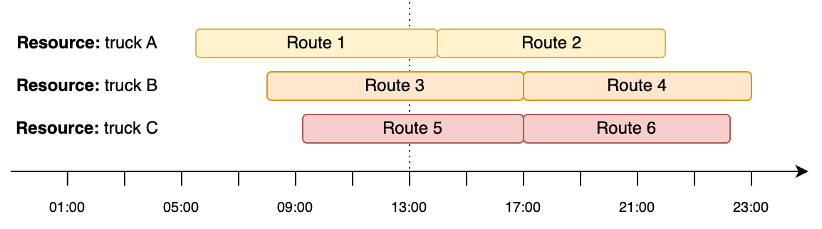
AM/PM planning with shared trucks
In this scenario, we need to plan two driver shifts, AM and PM, with each driver represented as a vehicle. Drivers have a maximum route duration (e.g., 9 hours) but no fixed operating hours, allowing the algorithm to schedule orders flexibly throughout the day based on their time slots. The challenge comes from the fact that the number of available trucks is limited and must be shared between both shifts.
To model this operational constraint, trucks are represented as resources required by vehicles. Since a truck cannot be used by two drivers at the same time, the optimization ensures that routes assigned to vehicles sharing the same truck do not overlap in time. This exclusivity prevents impossible simultaneous truck assignments while still allowing flexible scheduling of drivers’ routes.
The image below illustrates an example output for an AM/PM plan. Each row represents two drivers sharing a single truck. Since most of the work occurs after 13:00, manually splitting the vehicles into fixed shifts, AM drivers from 1:00 to 13:00 and PM drivers from 13:00 to 23:00, could have prevented certain orders from being planned or AM vehicles being underutilized.